"ASH math" of time_waited explained with pictures and simulation
As explained by John Beresniewicz, Graham Wood and Uri Shaft in their excellent overview ASH architecture and advanced usage, avg( v$active_session_history.time_waited ) is not a correct estimate of the average latency (the “true average”) esperienced by a wait event, the reason being that short events are less likely to be sampled. In order to correct this, the authors propose a formula that gives an unbiased estimate of the “true average”.
In this post I will quantitatively illustrate why sampling is so bad for time_waited, how the formula corrects it, and the sampling “distortion” of “reality” in general, by using an “ASH simulator” I have built and analyzing its data using basic statistic tools (and graphs). I hope that this might help others (as it has definitely helped myself) to better understand the formula and especially the characteristics of this fantastic tool of Oracle named ASH - the one that I use the most nowadays when tuning and troubleshooting, mined by almost every script of my toolbox.
All the code and spools are available here.
The simulator
Obviously implemented in PL/SQL, as all great things in life, this pipelined function produces a stream of events:
SQL> select ... from table( sim_pkg.events( ... ) );
SESSION_STATE  ELAPSED_USEC
------------- -------------
WAITING         180,759.713
ON CPU          500,000.000
WAITING         164,796.844
ON CPU          500,000.000
WAITING       2,068,034.610
ON CPU          500,000.000
WAITING       2,720,383.092
ON CPU          500,000.000
It simulates a process that alternates between consuming CPU and waiting for an event; the desired probability density functions of the two stochastic processes “on cpu” and “waiting” can be passed as arguments.
This stream can then be sampled by pipelining the stream to this other function:
SQL> select ...
      from table( sim_pkg.samples (
                    cursor( select * from table( sim_pkg.events( ... ) )
                )
     );
 SAMPLE_ID SAMPLE_TIME SESSION_STATE      TIME_WAITED
---------- ----------- ------------- ----------------
         0           0 WAITING            180,759.713
         1     1000000 ON CPU                    .000
         2     2000000 WAITING                   .000
         3     3000000 WAITING          2,068,034.610
         4     4000000 WAITING                   .000
         5     5000000 WAITING                   .000
         6     6000000 WAITING          2,720,383.092
         7     7000000 ON CPU                    .000
Note that the function also reproduces the artificial zeros introduced by ASH’s fix-up mechanism (i.e., event with time_waited = 2,720,383.092 spans three samples and hence has the two previous samples set to zero; same for its predecessor). Notice also that one “short” event has been missed by the reaping sampling hand.
Investigation by pictures
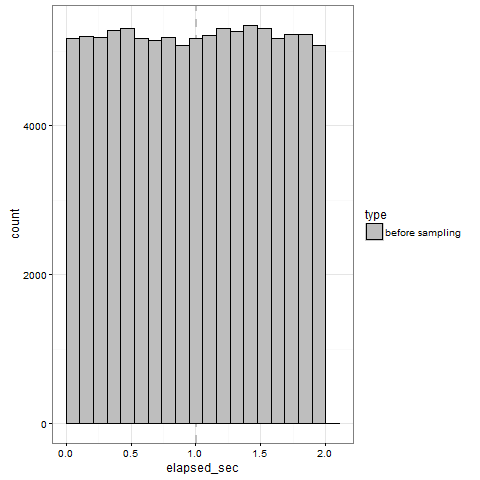
Let’s produce an event stream that follows an uniform distribution on the interval [0 .. 2 sec]; here is its histogram (produced by the wonderful geom_histogram() of R’s ggplot2 package):
So we can visually appreciate and confirm that all events are contained in the requested interval and respect the desired distribution; please also note that the average (the thin dashed vertical line) is almost perfectly equal to the expected value E[ events ] = 1.0.
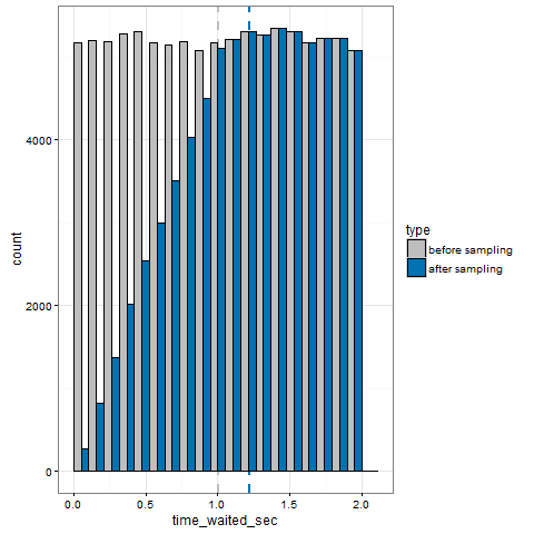
Let’s sample the stream, ignore the artificial zeros, and superimpose the samples’ histogram to the previous one:
So we can see that events longer then the sampling interval T (1sec) are always sampled and hence faithfully represented (the histograms bars match perfectly), but shorter events are not. For example, note that for time_waited = 0.5sec only half of the events are represented - in other words, the probability of being sampled is linearly proportional with time_waited.
More precisely, for time_waited < 1sec, the histogram height of the samples is equal to the histogram height of the events times k * time_waited, with k = 1 / T = 1 / (1.0sec); same for the pdf but with a different value for k. Let’s call this the “short waits distortion”.
Now check avg(time_waited), the dashed blue line: because of the bias of the samples towards higher values, it overestimates the “true average” by about 0.25 sec. It is actually an almost perfect estimation of the expected value of the samples, that can be calculated by integrating the pdf as being E[samples] = 11/9sec - that unfortunately is nothing we care about, but it confirms the correctness of our analysis.
From the above illustration, it is evident that avg(time_waited) is going to always be an overestimation, regardless of the pdf of the event stream. Hence, it can be never used reliably when tuning of analyzing.
ASH math to the rescue
Since the simulator is written in PL/SQL, we can plug it in place of v$ash in the formula of the unbiased estimator and check its output easily:
TIME_WAITED_AVG         TRUE_AVG TIME_WAITED_MATH_USEC ERR_PERC
--------------- ---------------- --------------------- --------
1221775.3          1,000,428.287         1,001,574.585      .11
So ASH math estimates about 1.001574 sec, extremely close to the true value of 1.000428 sec (an error of only 0.11%). Not bad at all!
The formula has been for sure derived using some statistical tool/theorem that I don’t know [yet ;)], but its algorithm can be understood intuitively as a way of reversing the above illustrated pdf “short waits distortion” by re-counting events accordingly.
In fact, avg(time_waited) for N samples is, by definition, the ratio of
numerator = sum of time_waited ( i )
denominator = N
The formula uses instead (assuming all time_waited < 1sec for simplicity)
numerator = sum of T = N * 1.0 sec
denominator = sum of T / time_waited ( i )
Note that in both cases the physical dimension of the numerator is time while the denominator is adimensional and has a physical meaning of counts.
The formula corrects the pdf distortion by assuming that, for each sample, we have T / time_waited(i) events in the original stream, all but one escaping the sampling hand (not necessarily in the current i-nth sampling interval, could be in another). E.g. for every observed sample of 0.1 sec there are actually 10 wait events in the original stream, 1 sampled, 9 missed - as we illustrated in the pretty pictures above.
Thus, for each observed sample, the “true” number of counts is not 1, but T / time_waited(i), for a total “true” waited time of time_waited(i) * counts = time_waited(i) * [T / time_waited(i)] = T. The formula then simply adds both “true” counts and “true” waited times for all samples.
I don’t know why this formula estimator is unbiased, its statistical properties in general and how it was derived - if someone has any information or tip, please chime in. A background but strong interest of mine is to better understand ASH to apply data-mining algorithms to my everyday’s tuning efforts, especially to produce prettier pictures ;)

